Ceramic Forum, Glass Manufacturing Technology and Wide-Gap Semiconductors
Improved DLTS Method
Measurement of junction capacitance change due to carrier emission from a deep level is the main point of the DLTS method, but in reality, this capacitance change is very small, in the sub fF to pF order
From the viewpoint of measurement technology, measurement of such a weak signal requires a method with a high S/N ratio.
Lang's method (Boxcar method) is actually an effective method for the measurement of very weak signals.
In actual measurement, transient measurement is performed repeatedly under one temperature, and S/N is improved by averaging output signals.
Since then, in the DLTS method to date, improvements have been made aimed at how to efficiently obtain highly sensitive data from very weak signals.
Lang's DLTS method was a so-called analog system.
Although it can be said that it was an ingenious method of extracting information from a high-speed signal in an era without high-performance computers, it was never an efficient method.
It can also be said that it only uses a small part of the transient signal information.
Today, now that it is easy to use high-performance personal computers, the situation is very different, and it is relatively simple technology to fully collect the transient signal in the range of μs to s in DLTS as digital data.
In the digital data system, for example, using one transient data, the operation of obtaining the temperature change of the time constant from the combination measurement of differing t1 and t2 can be done by software on the computer. Therefore, it is not necessary to perform a complicated measurement that repeatedly needs to lower / raise the temperature
On the other hand, the peak shape in the DLTS spectrum is basically broad, so it was never good from the viewpoint of level energy resolution.
In recent years, with the development of digital signal processing technology, innovations in the DLTS method aim for high resolution as well as high sensitivity.
For signal processing in PhysTech's DLTS device, analysis using various methods is possible such as Fourier transform method, correlation function method, Laplace transform method, multi-exponential fitting and deconvolution of ICTS spectrum and DLTS spectrum etc.
Especially, the method using Laplace transform in HERA-DLTS, provides analysis results with emphasis on energy resolution which were insufficient in the conventional DLTS method, adding new possibilities to the DLTS method.
Fourier transform DLTS
As early as 1982 there have been reports 4) of methods using Fourier transform for signal processing in DLTS, in particular one called DLTFS (Deep Level Transient Fourier Spectroscopy).
In the DLTFS method, it is possible to directly derive the time constant of the emission process at the temperature from the transient data."Direct" as used here means that it is not "Indirect" like the method of obtaining it from the peak of the spectrum (temperature dependent curve) in the general DLTS method.
The main points of this method 5) used for the current Phystech DLTS device are as follows.
- Perform discrete Fourier transform of N measured data in a capacitance transient, and determine its coefficient: CnD.
- Presume a carrier emission mechanism from the target deep level.For example, in the case of discrete levels in general point defects, it is a multi-exponential rate process like the following formula (A-16).
- Expand this formula by Fourier series, and calculate its coefficient: Cn.
- On the premise that CnD is based on the mechanism assumed in 2, the parameters contained in the latter formula are determined from the comparison of CnD and Cn , and parameters of deep level (activation energy, capture cross-section) and level concentration are obtained.
The multi-exponential time principle is expressed by the following formula.
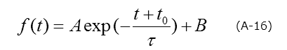
A: amplitude, B: offset, τ: time constant, to: sampling wait time
Also, its Fourier coefficient is expressed as follows.
Here, a and b represent the coefficients of cos (cosine) and sin (sine), respectively, in the Fourier series expansion. And n represents its degree.

The expression in the second row of the formulas (A-17) and (A-18) is normalized by τ / Tw. Therefore, the expression in the second row of the formulas (A-17) and (A-18) is normalized by t0 / Tw.
In addition, the following relation is arranged, and this is used to evaluate whether the transient is exponential or not.
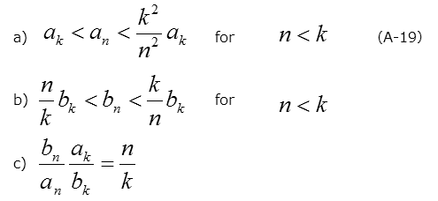
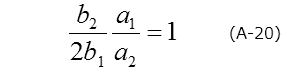
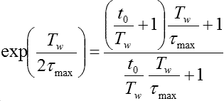
In particular, when using the 1st and 2nd degree coefficients, the following relationship is obtained and is used as an index to evaluate "exponential function class" in the FT1030 software.
In addition, the following relation is arranged, and this is used to evaluate whether the transient is exponential or not.
In addition, the following relation is arranged, and this is used to evaluate whether the transient is exponential or not.
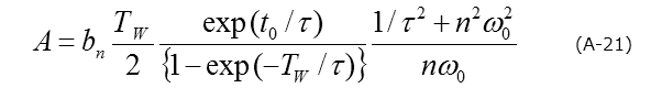
The amplitude in the transient waveform corresponds to the concentration of the deep level, but it is calculated from each Fourier coefficient.
For example, in the case of bn, it is expressed by the following formula
Now, the time constant is obtained from the ratio of two Fourier coefficients.There are three methods

Here, it can be said that it is a considerable advantage that the time constant is determined only by the ratio of the coefficients, regardless of the amplitude of the transient or the offset.
Correlation Function Method (or weighting function method)6-8)
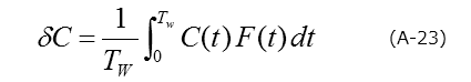
In this method, as shown in the following formula, multiply a capacitance transient waveform by a certain function (correlation function or correlator), integrate it over the measurement time range, and standardize it by that time.
Also, as the correlator, it is mainly selected as the one which yields to 0 (zero) when time integration is done over the interval of integration.
What is obtained here is considered as corresponding to the difference in the capacitance transients in Lang's method, as explained below.
Now, remember Lang's method.
The capacitance values C(t1) and C(t2) at two times t1 and t2 in the capacitive transient were measured and the difference S (T) = ΔC = (t1)-C(t2) determined.
Here, consider the delta function of F(t1)=1 and (t2) - 1, and apply the following correlator: F(t).
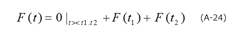
Calculate the formula (A-23) while using this correlator, and δC = C(t1)-C(t2)is obtained as a result.
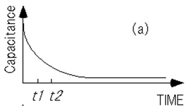
In other words, Lang's method can be thought of as a correlation function method with a correlator of delta function like formula (A-24) (Figure A-5).
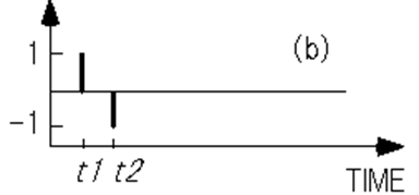
Figure A-5. Transient measurement by Lang (a) capacitance transient waveform, (b) delta function (Boxcar correlation function)
However, from the viewpoint of S/N ratio the Boxcar correlator was not a good correlator.
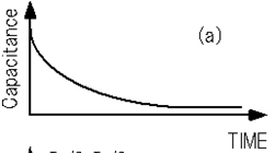
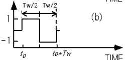
As a correlator, capable of improving the S / N ratio, there is the square wave function 8) as shown in Figure A-6 (b).
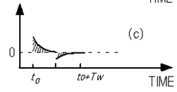
When this correlator is used for a capacitance transient waveform as shown in Figure A-6 (a), the calculation result of formula (A-23) is represented by the difference in the oblique shaded area, which is both sides of 0, as shown in Figure A-6 (c).
Also, from another point of view, since the square wave function is reversed in polarity from 1 to -1 between the time t0+Tw/2, the above difference in the area can also be said to be an average of the calculation results of the delta function type correlator in the interval of Tw/2.
Description of Correlation Function Method by Square Wave Function (a) capacitance transient waveform, (b) square wave correlator, (c) conceptual diagram of calculation results of formula (A-23)
Plot point δC in formula (A-23), as a function of temperature, is the DLTS spectrum in the correlation function method.
The temperature at the peak position that appears on the spectrum is the temperature that shows the time constant, Τmax, determined by the type of correlator, TW, and t0.
The relational expression is expressed by the following formula (A-25).
Although the maximum condition cannot directly set Τmax, but by giving the value of TW, t0 as a measurement condition, Τmax can be obtained by numerical calculation.
Now, from the concept of Fourier transform, the calculation for obtaining the above Fourier coefficients a and b, is actually equivalent to the correlation function method with cos and sin functions as correlators.
In particular, these primary coefficients a1 and b1 are used respectively as standard spectra (variables on the vertical axis) in the ”Periodwidthscan” and ”Tempscan” methods of the FT1030 software.
In the FT1030 software, 23 correlators including other higher degree Fourier coefficients and square wave functions are prep
By analyzing the DLTS spectrum by these correlators, a large number of Arrhenius plot points are obtained from a single tempscan (temperature scan) measurement.
In addition, various correlators have different characteristics regarding their sensitivity and resolution, and generally have a trade-off relationship between them. 9)
In short, high-sensitivity correlators tend to be inferior in energy resolution and vice versa.
Figure A-7 illustrates a typical correlator. 10)
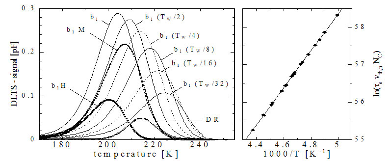
Also, Figure A-8 shows the DLTS spectra of these correlators and the Arrhenius plot of the data obtained from the peak positions in each spectrum.
Figure A-7.Correlator (correlation function) example
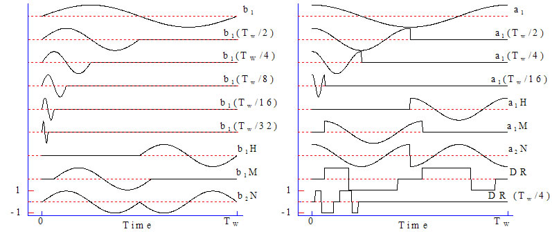
Figure A-8.
(Right) Comparison of DLTS spectra by various correlators
(Left) Arrhenius plot by data obtained from each peak position
Laplace transform method DLTS (LDLTS) method11,12)
The disadvantage of the conventional DLTS method, as described above, is that it was inferior in energy resolution.
As the photoluminescence spectrum measured at a low temperature has a fine structure composed of sharp exciton emission lines, information on the relevant energy level is obtained with high resolution
On the other hand, the DLTS spectrum generally gives only broad peaks without micro-structure.
If there are multiple levels with similar energy, it is difficult to separate and detect them.
The Laplace transform formula DLTS (LDLTS) method is an analysis method with emphasis on this energy resolution.
The LDLTS method is based on transient measurement under constant temperatures, like the ICTS method.
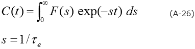
Considering the non-exponential nature, a transient is expressed as a continuous function of emission rate (= inverse number of a time constant) as in formula (A-26).
In other words, the spectral density function (distribution of the emission rate): F (s) is the Laplace transform of the capacitance transient.
To obtain the distribution function of the emission rate: F(s) from a capacitance transient is to be an inverse Laplace transformation, this is the "ill posed inverse problem" in mathematics, and it is impossible to immediately obtain unambiguous solutions from capacitive transient data, which is obtained experimentally.
On the other hand, the FT1030 uses software CONTIN (S. Provencher) 13) based on the Tikhonov regularization method which is a general solution to "ill posed inverse problems".
Again, several conditions are required to obtain the correct solution, but to conclude, it is known that a good S/N ratio, especially in transient data, is important.
It is estimated that S/N = 1000 is necessary to achieve the time constant ratio of two similar levels: Τ1/Τ2 ~ 2.
However, this condition is assumed to be experimentally possible, and considering the fact that Τ1/Τ2 are limited, up to about 12 and 15 respectively in the DLTS conventional Boxcar method and square wave function method, the LDLTS method can be said to be a very effective means for separating proximity levels.
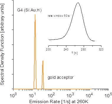
Figure A-9.LDLTS spectrum of the level related to Au in Si containing hydrogen (@ 260K).The inserted figure shows the spectrum by conventional DLTS method (rate window: 50 s-1), in the LDLTS spectrum, the existence of two levels with similar level energy is shown.
The sample is one obtained by introducing H (hydrogen) into Si that is diffused by Au (gold).
The inserted figure in the upper right is the spectrum (rate window = 50s-1) by the conventional DLTS method and has a typical broad peak around 260K.
This peak was known in the past as an acceptor level due to Au in Si.
On the other hand, the LDLTS spectrum (horizontal axis: emission rate) measured at 260 K observed two sharp peaks like δ function types.
Regarding these peaks, it has been reported that the low rate side is caused by the emission process from the level called G4 by the Au-H complex (Ea=542meV), and the high rate side is from the level of the Au acceptor itself (558 meV).
Conventional DLTS method was only able to recognize one peak (= one level), but in the LDLTS method it was shown that separation of such similar levels is possible.
In this way, the LDLTS method is a major feature of the high energy resolution that could not be achieved by the conventional DLTS method. However, due to the nature of the analysis, it is important to note that the vertical axis intensity of the spectrum does not reflect the trap concentration.
しConcerning the trap concentration, for example, analysis by the method like conventional DLTS method may be necessary.
In addition, there are several reasons why the DLTS peak broadens in the first place, and it is not necessarily the existence of proximity levels.
A typical example may be the influence on the emission rate by the local electric field around the defect (Poole-Frenkel effect) etc.
Therefore, do not forget that separating spectra does not always give correct results.
● References
4) K. Ikeda and H. Takaoka, Jpn. J. Appl. Phys. 21, 462 (1982).
5) S. Weiss and R. Kassing, Solid-State Electronics, 31, 1733 (1988).
6) G. L. Miller, L. V. Ramirez, and D. A. Robinson, J. Appl. Phys. 46, 2638 (1975).
7) L. C. Kimerling, IEEE Trans. Nucl. Sci. NS-23, 1497 (1976).
8) Y. Tokuda, N. Shimizu, and A. Usami, Jpn. J. Appl. Phys. 18, 309 (1979).
9) A. A. Istratov, J. Appl. Phys. 82, 2965 (1997).
10) E. Fretwurst, Workshop on Defects, Hamburg, August 23-2006.
11) L. Dobaczewski, P. Kaczor, L. D. Hswkins, and A. R. Peaker, J. Appl. Phys. 76, 194 (1994).
12) L. Dobaczewski, A. R. Peaker, and B. Nielsen, J. Appl. Phys. 96, 4689 (2004).
13) S. W. provencher, Comput. Phys. Commun. 27, 213 (1982).
14) P. Deixler et al., Appl. Phys. Lett., 73, 3126 (1998).